Rate of change of a value shows at which rate or velocity a value is changed over time. In industrial measurements ROC of a process parameter may be an indication of how rapidly the process evolves. Particularly, in power transformers dissolved gas analysis measurements ROC of gas concentrations can provide an information of the severity of the internal fault of the transformer.
Given the measured value dependency over time as a formula y=f(t), the ROC of y will be a derivative f’(t).
However, in a typical industrial application:
the f(t) formula is unknown;
measurement results are discrete in time;
measurement results contain a measurement uncertainty.
In such cases two ways to calculate the ROC are either by taking a simple ratio of the change in the process parameter to the change in time, or by using a linear fit method. Both approaches provide an approximation to the derivative. In this article we'll see how these methods are compared to each other and how precisely do they calculate the ROC.
In the first technique the ROC is quantified as the ratio of the change in the value to the change in time over a certain time window. In the image below, the ROC of the value in the point 2 is defined as:

Here the selected time window is set by t2-t1.

The second technique uses a linear approximation to calculate the ROC. For a linear function of the kind

proportional coefficient k is the tangent of the angle α between the linear fit line and the horizontal axis. In turn, this tangent is a ratio of the change in value to the change in time. Similar to the definition of ROC from the case above, this is an approximation of the ROC of a value. In the picture below for all the points within the selected time window a linear fit line is defined. So, the ROC value for point 2 is the tangent α value.

To see how these two techniques work we'll examine three cases:
f(t) formula is known and has a constant ROC value;
f(t) formula is known and has a ROC value known and changing over time;
f(t) formula and ROC value are both unknown.
We’ll also introduce a measurement instrument uncertainty since a measurement of an industrial process parameter always has to deal with some level of measurement error. This will introduce additional obstacle for a precise ROC calculation.
The process when f(t) is known and the ROC is constant can be described by this formula:

Here k is a constant value.
For such process the ROC is simply k and remains constant. Since our process is purely fictional, we'll take a k value of 0.1 whatever it could stand for.
We’ll assume the process is controlled by a sensor that has a measurement error 2. After it we’ll assume measurement results follows a three sigma rule. This means the measured values will have a normal distribution with the mean value being the true value and triple deviation being a measurement error. This means 99.7% of all measured values will not be farther than the measurement error from the true value.
The python code below generates our true and measured values and calculates both simple ratio and linear fit ROCs.
Here we’ll get a vector of true value as true_value and a vector of measured values measured_value for the time window from 0 to 500. To make it simpler, we’ll use dimensionless time units, since it doesn’t really matter for a fictional process whether to count time in seconds, hours or even days. true_value_roc is the true ROC which is 0.1 for our process. measured_value_roc1 and measured_value_roc2 are ROCs calculated by linear fit and simple ratio techniques. MA_WINDOW is the time window we’ll use to calculate ROCs.
With this setup a plot with the true and measured values looks like this:

Then, if we select a time frame (MA_WINDOW) as 10 time units, we’ll get these results for the simple ratio and linear fit ROCs:

The very beginning of both calculated ROCs plots are zeros since there’s simply not enough data to calculate them when time values are less than the selected time window.
Apparently both ROCs are not very precise. Several spikes in the simple ratio ROC can go up to 0.4 and to 0.3 for the linear fit ROC. If we then enlarge the time window to 50 time units, the results will be the following:

Here the results look better, however the “dead” zone at the beginning of the graphs got increased since there were not enough data to calculate ROC for the first 49 points. Spikes in the simple ratio ROC now reach only 0.15 and only about 0.11 for the linear fit ROC. Also, the linear fit ROC is much more smooth and does not fluctuate that rapidly as the simple ratio ROC.
After even more increasing the time window to 100 we’ll get these results:

Here the difference in both ROC is apparent. Simple ratio ROC provides less accurate results which fluctuate around the true value while linear fit ROC is more accurate and is changed much more smoothly.
The second case we’ll look at is when the process formula is known and the ROC is changing. A heating of a body can be a good example. Such process is described by the formula:

Here
T is the temperature of the body at the time moment t;
T0 is the initial temperature of the body;
Ts is the temperature of a surrounding media;
k is the constant.
Given this formula, the ROC is calculated simply:

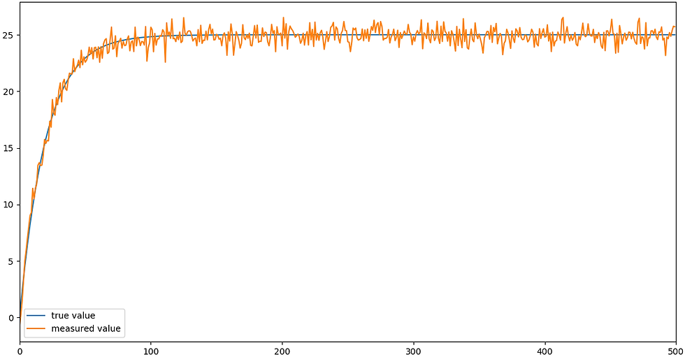
For our purely fictional process we'll assume the values in T and ROC formulas the following (as if a body having the temperature 0 deg.C is exposed to the environment with the temperature 25 deg.C):
Ts = 25
T0 = 0
k = 0.5
This Python code generates temperatures and ROC values:
Having the same measurement error 2, we’ll get the following trends for the true and measured temperatures:
Taking the time window as 10 time units, we’ll get this plot for both ROCs:

Like the previous case, both ROCs are not very precise with the simple ratio ROC fluctuating a bit more than the linear fit one.
With the time window increased to 50, the results are the following:

The accuracy is drastically bad right after the “dead” zone, where the measured value changed rapidly. When the actual ROC is flattened, both calculated ROCs accuracies keep at the decent level with, again, the simple ratio ROC fluctuating a bit more than the linear fit one.
When the time window is increased to 100, the results are the following:

Again, the calculated ROC accuracy is the worst right after the “dead” zone with the same reason - the measured value changed rapidly.
For the third case, when both f(t) and ROC are unknown, we'll generate a random time series using the random walk algorithm. The random walk algorithm generates a sequence of random steps in some mathematical space. Our space will be the one-dimensional space of true values. This means the random walk algorithm will be defined by the formula:

Here y(i) is the position after i-th step which is defined as the previous position y(i-1) and a random step. As a random step we’ll take a random value from the standard normal distribution (with mean 0 and variance 1).
Such vector of random values generated by the random walk algorithm can be assumed to be spread over time thus making it a random time series.
The Python code below generates such random walk time series and calculates both ROCs.
Random walk generated time series look like this:

A thing to note is that we didn’t apply the measurement uncertainty before calculating ROC because this ‘true value’ is already random in nature.
Having set the time window to 10 time units, two ROCs look like this:

They are almost identical with no much advances in accuracy or smoothness to spot.
With the time window set to 50, ROCs look like this:

And when the time window is 100, ROCs look like this:

It’s difficult to conclude which ROC provides better accuracy since the actual ROC is unknown, but we can see that the linear fit one is way more smooth than the simple ratio one.
As a conclusion, linear fit ROC seems to be a better choice for industrial applications as it provides seemingly better accuracy and is less subjected to random changes in measured values. Linear fit ROC is more straightforward and can be easier to calculate. Both ROCs show better accuracy when more measurements are comprised by the selected time window.
List of sources
Github repository with the code used to generate plots in this article https://github.com/leonidpospeev/roc-calculation
Wikipedia: 68-95-99.7 rule https://en.wikipedia.org/wiki/68%E2%80%9395%E2%80%9399.7_rule
Wikipedia: Random walk algorithm https://en.wikipedia.org/wiki/Random_walk
Комментарии